Child mortality rate, 1960 to 2021

Author

math4mad

ref

ref : Child mortality rate, 1960 to 2021
package :The newggslopegraph function from the CGPfunctions package

Code

 include("utils.jl")

[ Info: loading success

Code

make_title("Part one : Data processing")

Part one : Data processing

load csv

Code

df=@pipe CSV.File("./data/child-mortality-1960-vs-latest-slope.csv")|>DataFrame|>rename(_,"Observation value - Unit_of_measure: Deaths per 100 live births - Indicator: Under-five mortality rate - Sex: Both sexes - Wealth_quintile: All wealth quintiles"=>:rate)|>select(_,Not(:Code,:Continent,"Population (historical estimates)"))|>dropmissing

13472×3 DataFrame

13447 rows omitted

Row	Entity	Year	rate
	String	Int64	Float64
1	Afghanistan	1957	37.5905
2	Afghanistan	1958	36.9628
3	Afghanistan	1959	36.3437
4	Afghanistan	1960	35.7301
5	Afghanistan	1961	35.1658
6	Afghanistan	1962	34.584
7	Afghanistan	1963	34.0159
8	Afghanistan	1964	33.4848
9	Afghanistan	1965	32.9421
10	Afghanistan	1966	32.3938
11	Afghanistan	1967	31.8366
12	Afghanistan	1968	31.2825
13	Afghanistan	1969	30.7243
⋮	⋮	⋮	⋮
13461	Zimbabwe	2010	8.61062
13462	Zimbabwe	2011	8.05877
13463	Zimbabwe	2012	7.21463
13464	Zimbabwe	2013	6.62226
13465	Zimbabwe	2014	6.26086
13466	Zimbabwe	2015	6.04718
13467	Zimbabwe	2016	5.78704
13468	Zimbabwe	2017	5.61751
13469	Zimbabwe	2018	5.36877
13470	Zimbabwe	2019	5.26659
13471	Zimbabwe	2020	5.17696
13472	Zimbabwe	2021	4.9522

tidy data

Code

  query_years=[1960,1980,2000,2020]
  query_countries=["Abkhazia","Uganda","Kenya","Egypt","Spain","Japan","France"]
  @eval(Main, input_years=query_years)
  @eval(Main, input_countries =query_countries)
  @eval(Main,input_points=length(query_years))
  df=@chain df begin
      @filter(Year ∈ !!input_years)
      @group_by(Entity)
      #filter(d->nrow(d)==4,_) 
      @filter(length(Year)==!!input_points) 
      @arrange(Year)
      @ungroup
      coerce(_,  :Year=>OrderedFactor)
      @mutate(rate=round(rate,digits=1))
      @filter(Entity ∈ !!input_countries)
  end

24×3 DataFrame

Row	Entity	Year	rate
	String	Cat…	Float64
1	Egypt	1960	31.8
2	Egypt	1980	16.8
3	Egypt	2000	4.7
4	Egypt	2020	2.0
5	France	1960	2.8
6	France	1980	1.2
7	France	2000	0.5
8	France	2020	0.4
9	Japan	1960	4.0
10	Japan	1980	1.0
11	Japan	2000	0.5
12	Japan	2020	0.2
13	Kenya	1960	19.7
14	Kenya	1980	11.1
15	Kenya	2000	9.9
16	Kenya	2020	3.9
17	Spain	1960	5.5
18	Spain	1980	1.5
19	Spain	2000	0.5
20	Spain	2020	0.3
21	Uganda	1960	22.3
22	Uganda	1980	21.9
23	Uganda	2000	14.6
24	Uganda	2020	4.4

Code

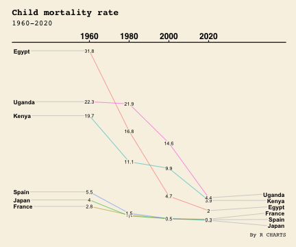
make_title("Part 2:  Plot")

Part 2: Plot

Code

  @rput df
  R"""
    # install.packages("CGPfunctions")
     library(CGPfunctions)
     newggslopegraph(dataframe = df,
                Times = Year,
                Measurement = rate,
                Grouping = Entity,
                Title = "Child mortality rate",
                SubTitle = "1960-2020",
                Caption = "By R CHARTS",
                LineThickness = 0.5,
                # DataLabelPadding =0.2,
                # DataLabelLineSize = 0.5,
                # DataLabelFillColor = "lightblue",
                ThemeChoice = "wsj"
                )
  """

RObject{VecSxp}