Code
    include("../utils.jl")
    import MLJ:fit!,fitted_params
using GLMakie,MLJ,CSV,DataFramesGLMakie:contourf 方法 include("../utils.jl")
import MLJ:fit!,fitted_params
using GLMakie,MLJ,CSV,DataFramesiris = load_iris();
#selectrows(iris, 1:3) |> pretty
iris = DataFrames.DataFrame(iris);
first(iris,5)|>display
y, X = unpack(iris, ==(:target); rng=123);
X=select!(X,3:4)
byCat = iris.target
categ = unique(byCat)
colors1 = [:orange,:lightgreen,:purple];| Row | sepal_length | sepal_width | petal_length | petal_width | target |
|---|---|---|---|---|---|
| Float64 | Float64 | Float64 | Float64 | Cat… | |
| 1 | 5.1 | 3.5 | 1.4 | 0.2 | setosa |
| 2 | 4.9 | 3.0 | 1.4 | 0.2 | setosa |
| 3 | 4.7 | 3.2 | 1.3 | 0.2 | setosa |
| 4 | 4.6 | 3.1 | 1.5 | 0.2 | setosa |
| 5 | 5.0 | 3.6 | 1.4 | 0.2 | setosa |
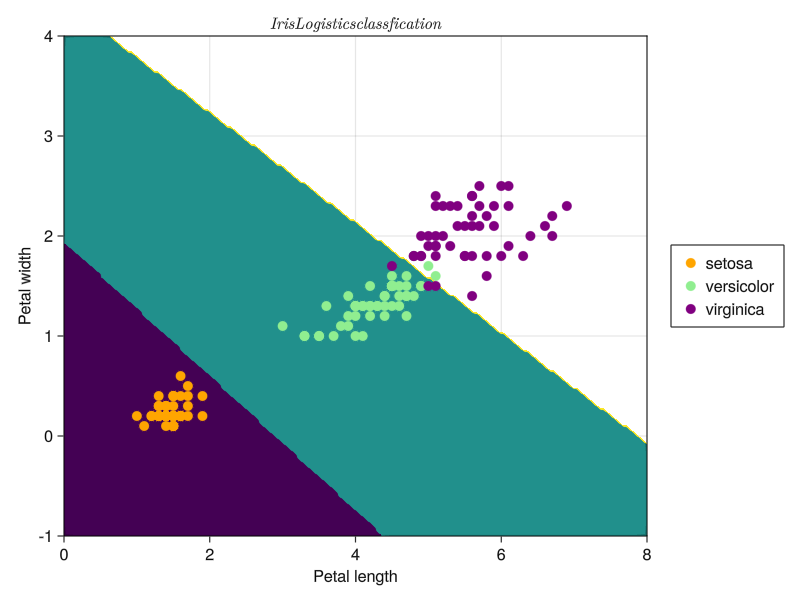
生成决策边界实际是利用训练模型对区间内的每个点都做出预测,利用两个属性的最大值和最小值 生成 grid 数据,这是
test数据
# grid data
   n1 = n2 = 200
   tx = LinRange(0, 8, 200)
   ty = LinRange(-1, 4, 200)
   X_test = mapreduce(collect, hcat, Iterators.product(tx, ty))
   X_test = MLJ.table(X_test')
Tables.MatrixTable{LinearAlgebra.Adjoint{Float64, Matrix{Float64}}} with 40000 rows, 2 columns, and schema:
:x1 Float64
:x2 Float64 LogisticClassifier = @load LogisticClassifier pkg=MLJLinearModels
model = machine(LogisticClassifier(), X,y )
fit!(model)import MLJLinearModels ✔[ Info: For silent loading, specify `verbosity=0`.
[ Info: Training machine(LogisticClassifier(lambda = 2.220446049250313e-16, …), …).
┌ Info: Solver: MLJLinearModels.LBFGS{Optim.Options{Float64, Nothing}, NamedTuple{(), Tuple{}}}
│ optim_options: Optim.Options{Float64, Nothing}
└ lbfgs_options: NamedTuple{(), Tuple{}} NamedTuple()trained Machine; caches model-specific representations of data
model: LogisticClassifier(lambda = 2.220446049250313e-16, …)
args:
1: Source @794 ⏎ Table{AbstractVector{Continuous}}
2: Source @579 ⏎ AbstractVector{Multiclass{3}}ŷ = MLJ.predict(model, X_test)
res=mode.(ŷ)|>d->reshape(d,200,200)
function trans(i)
if i=="setosa"
res=1
elseif i=="versicolor"
res=2
else
res=3
end
end
ypred=[trans(res[i,j]) for i in 1:200, j in 1:200]200×200 Matrix{Int64}:
1 1 1 1 1 1 1 1 1 1 1 1 1 … 2 2 2 2 2 2 2 2 2 2 2 2
1 1 1 1 1 1 1 1 1 1 1 1 1 2 2 2 2 2 2 2 2 2 2 2 2
1 1 1 1 1 1 1 1 1 1 1 1 1 2 2 2 2 2 2 2 2 2 2 2 2
1 1 1 1 1 1 1 1 1 1 1 1 1 2 2 2 2 2 2 2 2 2 2 2 2
1 1 1 1 1 1 1 1 1 1 1 1 1 2 2 2 2 2 2 2 2 2 2 2 2
1 1 1 1 1 1 1 1 1 1 1 1 1 … 2 2 2 2 2 2 2 2 2 2 2 2
1 1 1 1 1 1 1 1 1 1 1 1 1 2 2 2 2 2 2 2 2 2 2 2 2
1 1 1 1 1 1 1 1 1 1 1 1 1 2 2 2 2 2 2 2 2 2 2 2 2
1 1 1 1 1 1 1 1 1 1 1 1 1 2 2 2 2 2 2 2 2 2 2 2 2
1 1 1 1 1 1 1 1 1 1 1 1 1 2 2 2 2 2 2 2 2 2 2 2 2
1 1 1 1 1 1 1 1 1 1 1 1 1 … 2 2 2 2 2 2 2 2 2 2 2 2
1 1 1 1 1 1 1 1 1 1 1 1 1 2 2 2 2 2 2 2 2 2 2 2 2
1 1 1 1 1 1 1 1 1 1 1 1 1 2 2 2 2 2 2 2 2 2 2 2 2
⋮ ⋮ ⋮ ⋱ ⋮ ⋮
2 2 2 2 2 2 2 2 2 2 2 2 2 3 3 3 3 3 3 3 3 3 3 3 3
2 2 2 2 2 2 2 2 2 2 2 2 2 3 3 3 3 3 3 3 3 3 3 3 3
2 2 2 2 2 2 2 2 2 2 2 2 2 … 3 3 3 3 3 3 3 3 3 3 3 3
2 2 2 2 2 2 2 2 2 2 2 2 2 3 3 3 3 3 3 3 3 3 3 3 3
2 2 2 2 2 2 2 2 2 2 2 2 2 3 3 3 3 3 3 3 3 3 3 3 3
2 2 2 2 2 2 2 2 2 2 2 2 2 3 3 3 3 3 3 3 3 3 3 3 3
2 2 2 2 2 2 2 2 2 2 2 2 2 3 3 3 3 3 3 3 3 3 3 3 3
2 2 2 2 2 2 2 2 2 2 2 2 2 … 3 3 3 3 3 3 3 3 3 3 3 3
2 2 2 2 2 2 2 2 2 2 2 2 2 3 3 3 3 3 3 3 3 3 3 3 3
2 2 2 2 2 2 2 2 2 2 2 2 2 3 3 3 3 3 3 3 3 3 3 3 3
2 2 2 2 2 2 2 2 2 2 2 2 2 3 3 3 3 3 3 3 3 3 3 3 3
2 2 2 2 2 2 2 2 2 2 2 2 2 3 3 3 3 3 3 3 3 3 3 3 3 function add_legend(axs)
Legend(fig[1,2], axs,"Label";width=100,height=200)
end
function desision_boundary(ax)
axs=[]
for (k, c) in enumerate(categ)
indc = findall(x -> x == c, byCat)
#@show indc
x=scatter!(iris[:,3][indc],iris[:,4][indc];color=colors1[k],markersize=14)
push!(axs,x)
end
return axs
end
fig = Figure(resolution=(800,600))
ax=Axis(fig[1,1],xlabel="Petal length",ylabel="Petal width",title=L"Iris Logistics classfication")
contourf!(ax,tx, ty, ypred, levels=length(categ))
axs=desision_boundary(ax)
Legend(fig[1,2],[axs...],categ)
fig