2-ecommerce-linear-reg

简介

通过上网浏览时间预测年花费

dataset: kaggle ecommerce dataset
model
using MLJLinearModels.jl 🔗

1. load package

Code

import MLJ:predict
using GLMakie, MLJ,CSV,DataFrames,StatsBase

WARNING: using StatsBase.predict in module Main conflicts with an existing identifier.

2. process data

Code

str="Ecommerce-Customers"   
df=CSV.File("./data/Ecommerce-Customers.csv") |> DataFrame |> dropmissing;
select!(df,4:8)
X=df[:,1:4]|>Matrix|>MLJ.table
y=Vector(df[:,5])
first(df,5)

5×5 DataFrame

Row	Avg. Session Length	Time on App	Time on Website	Length of Membership	Yearly Amount Spent
	Float64	Float64	Float64	Float64	Float64
1	34.4973	12.6557	39.5777	4.08262	587.951
2	31.9263	11.1095	37.269	2.66403	392.205
3	33.0009	11.3303	37.1106	4.10454	487.548
4	34.3056	13.7175	36.7213	3.12018	581.852
5	33.3307	12.7952	37.5367	4.44631	599.406

3. plot corrleation of variables

Code

axs = []
label=names(df)|>Array
colors = [:orange, :lightgreen, :purple,:lightblue,:red,:green]

fig = Figure(resolution=(1400, 1400))
ax=Axis(fig[1,1])

function plot_diag(i)

    ax = Axis(fig[i, i])
    push!(axs, ax)
    density!(ax, df[:, i]; color=(colors[i], 0.5),
            strokewidth=1.25, strokecolor=colors[i])
end


function plot_cor(i, j)
    ax = Axis(fig[i, j])
    scatter!(ax, df[:, i], df[:, j]; color=colors[j])
end


function plot_pair()
    [(i == j ? plot_diag(i) : plot_cor(i, j)) for i in 1:5, j in 1:5]
end

function add_xy_label()
    for i in 1:5
        Axis(fig[5, i], xlabel=label[i],)
        Axis(fig[i, 1], ylabel=label[i],)
    end
end

function main()

    plot_pair()
    add_xy_label()
    return fig
end

main()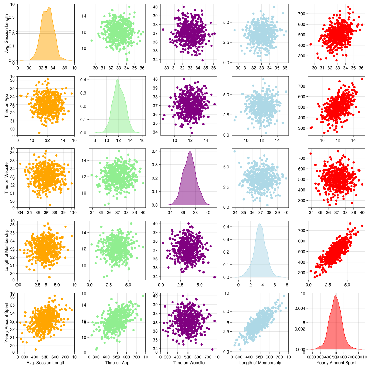

4. plot pair variables’s cov and cor matrix

Code

df_cov = df|>Matrix|>cov.|> d -> round(d, digits=3)
df_cor = df|>Matrix|>cor.|> d -> round(d, digits=3)

function plot_cov_cor()
    fig = Figure(resolution=(2200, 800))
    ax1 = Axis(fig[1, 1]; xticks=(1:5, label), yticks=(1:5, label), title="ecommerce cov matrix",yreversed=true)
    ax3 = Axis(fig[1, 3], xticks=(1:5, label), yticks=(1:5, label), title="ecommerce cor matrix",yreversed=true)

    hm = heatmap!(ax1, df_cov)
    Colorbar(fig[1, 2], hm)
    [text!(ax1, x, y; text=string(df_cov[x, y]), color=:white, fontsize=18, align=(:center, :center)) for x in 1:5, y in 1:5]

    hm2 = heatmap!(ax3, df_cor)
    Colorbar(fig[1, 4], hm2)
    [text!(ax3, x, y; text=string(df_cor[x, y]), color=:white, fontsize=18, align=(:center, :center)) for x in 1:5, y in 1:5]

    fig
end

plot_cov_cor()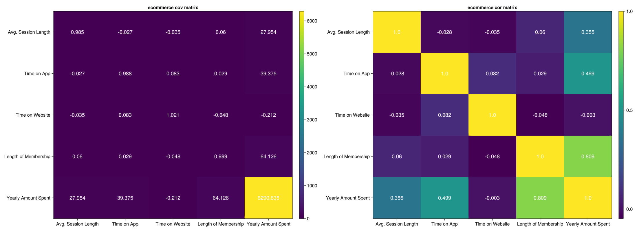

5. MLJ workflow

5.1 load model

Code

  LinearRegressor = @load LinearRegressor pkg=MLJLinearModels
  model=LinearRegressor()
  mach = MLJ.fit!(machine(model,X,y))
  fitted_params(mach)

[ Info: For silent loading, specify `verbosity=0`. 
[ Info: Training machine(LinearRegressor(fit_intercept = true, …), …).
┌ Info: Solver: MLJLinearModels.Analytical
│   iterative: Bool false
└   max_inner: Int64 200

import MLJLinearModels ✔

(coefs = [:x1 => 25.734271084705085, :x2 => 38.709153810834366, :x3 => 0.43673883559434407, :x4 => 61.57732375487839],
 intercept = -1051.5942553006273,)

5.2 predict

Code

  y_hat =predict(mach, X)
  "rmsd"=>rmsd(y,y_hat)

"rmsd" => 9.923256785022247

5.3 plot residuals

Code

resid=y_hat.=y
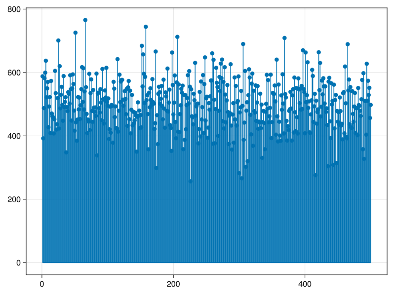
stem(resid)