1-kmeans-on-digits

简介

routine: project data to 2d space then proceed kmeans methods

1. ref: K-Means clustering on the handwritten digits data
2. kmeans in mlj
3. decision boundary:Prediction

1. load package

  include("../utils.jl")
  import MLJ: fit!, predict, transform,fitted_params
  using CSV, DataFrames, GLMakie, Random
  using MLJ
  Random.seed!(34343)

TaskLocalRNG()

2. load data

  load_csv(str::AbstractString) =
    str |> d -> CSV.File("./data/$str.csv") |> DataFrame |> dropmissing

  digits = load_csv("scikit_digits")
  digits = coerce(digits, :target => Multiclass)
  y, X = unpack(digits, ==(:target); rng = 123);

3. MLJ workflow

3.1 load model

  PCA = @load PCA pkg = MultivariateStats
  KMeans = @load KMeans pkg = Clustering
  pca_model = PCA(; maxoutdim = 2)
  kmeans_model = KMeans(; k =9)

import MLJMultivariateStatsInterface ✔
import MLJClusteringInterface ✔

[ Info: For silent loading, specify `verbosity=0`. 
[ Info: For silent loading, specify `verbosity=0`. 

KMeans(
  k = 9, 
  metric = Distances.SqEuclidean(0.0), 
  init = :kmpp)

3.2 usa pca model project data to 2d space

  pca_mach = machine(pca_model, X) |> fit!
  Xproj = transform(pca_mach, X)

[ Info: Training machine(PCA(maxoutdim = 2, …), …).

1797×2 DataFrame

1772 rows omitted

Row	x1	x2
	Float64	Float64
1	2.53068	7.10818
2	-7.06737	2.69455
3	9.71838	16.8406
4	2.73069	10.0099
5	-13.1702	-13.6058
6	-13.2824	8.86115
7	15.9065	-16.5451
8	-17.972	-7.82244
9	-5.2641	9.30009
10	-11.3988	-5.1612
11	-0.171222	-5.94507
12	6.49767	-25.2878
13	-27.8753	-5.61827
⋮	⋮	⋮
1786	18.7481	-2.69052
1787	18.0899	2.95523
1788	-16.321	7.03648
1789	-19.6796	0.109262
1790	19.5261	5.59811
1791	1.32969	-4.05499
1792	1.38873	2.25902
1793	2.15727	-4.79302
1794	-10.5746	2.93352
1795	-11.7413	-11.0562
1796	5.0894	-6.87343
1797	20.9178	1.59327

3.3 project decision data to 2d space

function boundary_data(df::AbstractDataFrame,;n=200)
    n1=n2=n
    xlow,xhigh=extrema(df[:,:x1])
    ylow,yhigh=extrema(df[:,:x2])
    tx = range(xlow,xhigh; length=n1)
    ty = range(ylow,yhigh; length=n2)
    x_test = mapreduce(collect, hcat, Iterators.product(tx, ty));
    xtest=MLJ.table(x_test')
    return tx,ty, xtest
end

 tx,ty, xtest=boundary_data(Xproj)

(-31.16990412454417:0.3159297962408993:31.70012532739479, -30.0922050904867:0.2893801640107357:27.494447547649695, Tables.MatrixTable{LinearAlgebra.Adjoint{Float64, Matrix{Float64}}} with 40000 rows, 2 columns, and schema:
 :x1  Float64
 :x2  Float64)

3.4 kmean flow

  kmeans_mach= machine(kmeans_model, Xproj) |> fit!

  ypred= predict(kmeans_mach, xtest)|>Array|>d->reshape(d,200,200)

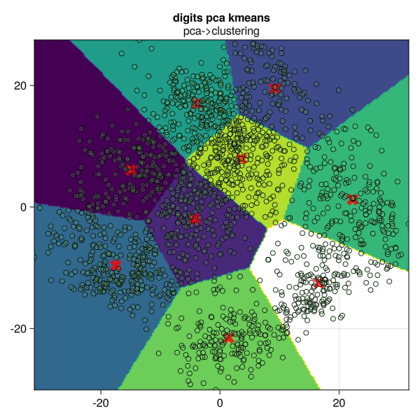
  cen=fitted_params(kmeans_mach)  #获取各聚类中心坐标

[ Info: Training machine(KMeans(k = 9, …), …).

(centers = [-14.940039081327807 -4.21080988089939 … 3.623938350681804 16.636412339611788; 6.0940188803548185 -1.9858645156958448 … 7.9454732936643895 -12.507323610991511],)

4. plot results

function plot_res()
    fig = Figure(resolution=(600,600))
    ax = Axis(fig[1, 1],title="digits pca kmeans",subtitle="pca->clustering")
    contourf!(ax, tx,ty,ypred)
    scatter!(ax,eachrow(cen.centers)...;marker=:xcross,markersize = 24,color=(:red,0.8))
    scatter!(ax,eachcol(Xproj)...;markersize = 8,color=(:lightgreen,0.1),strokecolor = :black, strokewidth =1)
    fig
end
plot_res()